There's no doubt that lattice-based cryptography is currently the most promising branch of post-quantum cryptography. Not only is it highly performant and versatile, it also provides the only known technique to achieve fully homomorphic encryption.

One reason lattice-based cryptography is so fast is that it can be heavily vectorized. This contrasts noticeably with isogeny-based cryptography, which offers far fewer opportunities for parallelism. In this post, I will briefly compare the potential for vectorization in both cryptographic paradigms. Of course, these two branches represent only a subset of the broader landscape of post-quantum cryptography.

Let's first take a look at what vectorization is.

Vectorization

Vectorization refers to the process of performing multiple operations simultaneously using Single Instruction, Multiple Data (SIMD) techniques. This is a powerful way to speed up computations by leveraging modern CPU instructions like SSE (Streaming SIMD Extensions), AVX (Advanced Vector Extensions), and their newer versions like AVX-512.

But what does that mean, really?

Let's say we would like to XOR 32 bytes as given below:

Input:  11001010 10101100 00011011 ...
Key  :  10110110 01100100 11100011 ...
---------------------------------
Output: 01111100 11001000 11111000 ...

Instead of doing 32 operations one byte at a time, AVX can XOR 32 bytes at once:

__m256i data  = _mm256_loadu_si256(input)
__m256i key   = _mm256_loadu_si256(key)
__m256i hash  = _mm256_xor_si256(data, key)

First, the AVX2 register uses input to load 32 bytes (256 bits) into one 256-bit register. Then, it loads 32 bytes of key into another register. Finally, it performs bitwise XOR between data and key, element by element. But here, 32 bytes are processed in one instruction!

Lattice-based cryptography

At the core of lattice-based cryptography lies matrix-vector multiplication. For example, let's consider a two-dimensional lattice $L$ with a basis $\{v_1, v_2\}$. Lattice elements are vectors of the form $a_1 v_1 + a_2 v_2$, where $a_1, a_2 \in \mathbb{Z}$. If we construct a matrix $M$ such that $v_1$ and $v_2$ are the two columns of this matrix, then multiplying $M$ by the vector $(a_1, a_2)^T$ gives a lattice element.

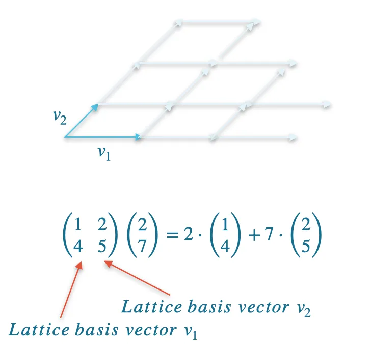
Matrix multiplication illustration

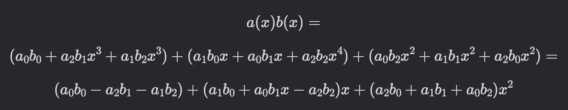
For performance reasons, lattice-based cryptography relies on polynomial rings rather than ordinary vectors. I won’t go into the details, but let’s consider the following example.

The matrix-vector multiplication above is actually the multiplication of two polynomials

in the ring $\mathbb{Z}[x]/(x^3 + 1)$. Note that in this ring, it holds $x^3 = -1$. In practice, $n$ is typically a power of $2$, for example $n = 64$.

So, multiplying $a(x)$ and $b(x)$ and considering $x^3 = -1$, we obtain the same result as with the matrix-vector multiplication above:

Having matrices of this form is beneficial for two reasons: less space is required to store the matrix (only $3$ elements for a $3 \times 3$ matrix), and we can apply the Number Theoretic Transform (NTT) algorithm for polynomial multiplication instead of performing matrix-vector multiplication. When using the NTT, we multiply polynomial evaluations rather than working with polynomial coefficients, which reduces the complexity from $O(n^2)$ to $O(n \log n)$ operations.

That means that instead of directly multiplying the polynomials

as

we apply the NTT to compute the evaluations $a(\omega_1), …, a(\omega_n)$ and $b(\omega_1), …, b(\omega_n)$. This allows us to perform only $n$ pointwise multiplications, significantly improving efficiency:

This way we obtain the evaluations of $a(x)b(x)$ at $\omega_1, ..., \omega_n$. To recover the coefficients of $a(x)b(x)$, we apply the inverse NTT. In the next section, we will see how vectorization can further accelerate such pointwise operations.

Lattices and vectorization

So, why is lattice-based cryptography particularly well-suited for vectorization?

Remember, typically lattice-based cryptography deals with polynomials in $\mathbb{Z}[x]/(x^{64}+1)$ or $\mathbb{Z}[x]/(x^{128}+1)$. For $n = 64$, each polynomial has $64$ coefficients, for example:

Now, if you want, for example, to compute $a(x) + b(x)$, you need to compute

This is simple to vectorize: we need to load $a_i$ and $b_i$ into an AVX register. Suppose the register has $32$ slots, each of length 16 bits. If the coefficients are smaller than 16 bits, we can use two registers for a single polynomial. With a single instruction, we compute the sum of the first $32$ coefficients:

a_1  | a_2  | ... | a_31 |
b_1  | b_2  | ... | b_31 |
->
a_1 + b_1  | a_2 + b_2  | ... | a_31 + b_31 |

In the second instruction, we compute the sum of the next $32$ coefficients:

a_32 | a_33 | ... | a_63 |
b_32 | b_33 | ... | b_63 |
->
a_32 + b_32 | a_33 + b_33 | ... | a_63 + b_63 |

Many lattice-based schemes heavily rely on matrix-vector multiplications, and similar to the approach above, these operations can be naturally expressed using vectorized instructions. Returning to the NTT, we see that these two polynomials can be multiplied efficiently using vectorization in just two instructions (performing 32 pointwise multiplications in a single instruction), along with the NTT and its inverse.

Isogenies and vectorization

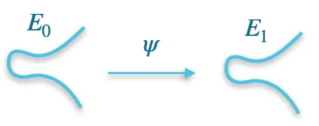
On the contrary, vectorizing isogeny-based schemes appears to be challenging. An isogeny is a homomorphism between two elliptic curves, and isogeny-based cryptography relies on the assumption that finding an isogeny between two given curves is difficult.

In isogeny-based cryptography, there are no structures with $64$ or $128$ elements that would allow straightforward vectorization. The optimizations used in isogeny-based cryptography are similar to those in traditional elliptic curve cryptography. Note, however, that traditional elliptic curve cryptography based on the discrete logarithm problem is not quantum-safe, while isogeny-based cryptography is believed to be quantum-safe: there is no known quantum algorithm that can efficiently find an isogeny between two elliptic curves.

Let's have a look at some optimizations used in elliptic curve cryptography:

• Choosing the prime $p$ such that the arithmetic in $\mathbb{F}_p$ is efficient,
• Montgomery Reduction: efficiently computes modular reductions without expensive division operations,
• Montgomery Inversion: avoids divisions entirely when used with Montgomery multiplication,
• Using Montgomery or Edwards curves: enables efficient arithmetic,
• Shamir’s Trick: computes $kP+mQ$ simultaneously, reducing the number of operations.

It is worth noting that some of these optimizations—such as Montgomery reduction and Montgomery multiplication—also apply to lattice-based cryptography.

Let's observe a simple example that illustrates the importance of choosing a suitable prime $p$ for efficient finite field arithmetic. If we choose $p \equiv 3\pmod{4}$ (that means $p+1$ is divisible by $4$), then computing square roots becomes straightforward: to find the square root of $x$, one simply computes:

Note that by Fermat's Little Theorem, it holds that $x^p = x \pmod{p}$, which means:

Elliptic curve operations can be vectorized but to a lesser extent as lattice-based operations. One example is handling field elements in radix-$2^{29}$ representation:

where $0 \leq f_i < 2^{29}$ for $0 \leq i \leq 8.$

However, the number of lanes plays a crucial role in SIMD optimizations. In lattice-based cryptography, it is straightforward to have $64$ or $128$ lanes, which can significantly enhance parallel processing capabilities. In contrast, the example above only utilizes $9$ lanes, which limits the potential for SIMD optimization.

Conclusion

Lattice-based cryptography is currently at the forefront of post-quantum cryptographic advancements, with performance being one of the key reasons for its prominence. Somewhat unjustly, isogeny-based cryptography has gained a reputation for being broken in recent years. This is due to the Castryck-Decru attack, which, however, applies only to schemes that expose additional information about the isogeny, namely the image of two points:

Given the images of two points under an isogeny $\psi$, one can compute the images of other points as well. For this, Kani's lemma, a remarkable result from 1997, is used. Thankfully, many isogeny-based schemes do not expose the images of points. One such example is SQIsign, which features super-compact keys and signatures, making them comparable in size to those used in elliptic-curve-based signature schemes. In summary, isogeny-based cryptography is less performant and less versatile than lattice-based cryptography; however, it offers advantages such as significantly smaller keys and signatures.

It will be interesting to see which area of post-quantum cryptography emerges as the dominant choice in the coming years. I haven't explored code-based, multivariate, or hash-based cryptography in depth yet, and each of these approaches comes with its own strengths and challenges.